Monte Carlo Analysis
Learn about Monte Carlo Analysis for real estate investing.
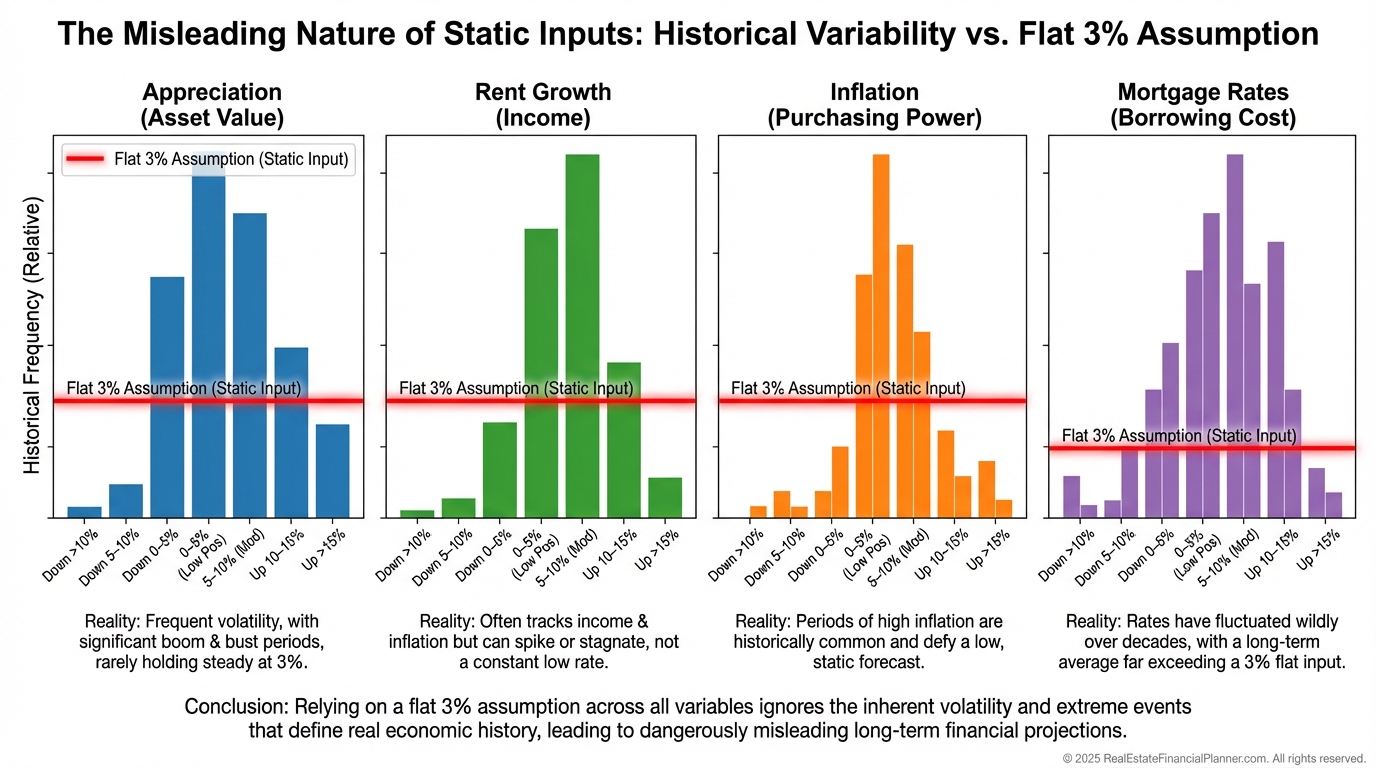
Why Static Assumptions Break
We all love clean spreadsheets, but the world refuses to cooperate.
When I help clients build plans in the Real Estate Financial Planner™ software, I never freeze appreciation at 3% and call it “true.”
History doesn’t move in straight lines.
Some years property values jump more than 10%. Some years they fall 5–15%.
Rents do it too.
Inflation drifts and spikes. Mortgage rates are a moving target until you lock. The stock market rarely hands you a steady 8%.
Using one number for each input hides risk, timing, and the range of possible futures.
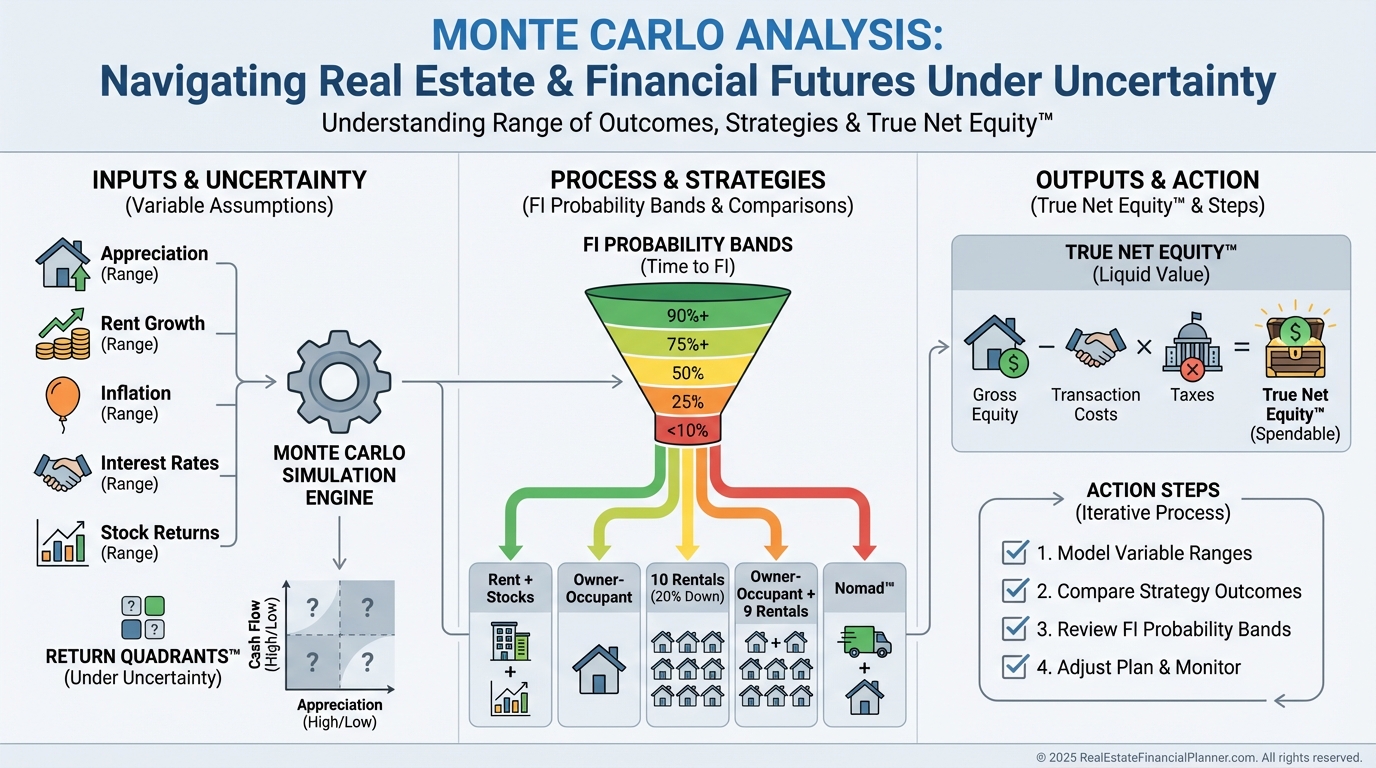
What Monte Carlo Analysis Is
Monte Carlo Analysis simulates hundreds or thousands of alternate futures.
Each run pulls a new path for appreciation, rents, inflation, rates, and market returns.
Then we analyze the distribution of outcomes: best case, worst case, median, and how often you hit your goals on time.
I call it Alternate Universe Modeling™ because it answers: “What happens to my plan across many plausible futures?”
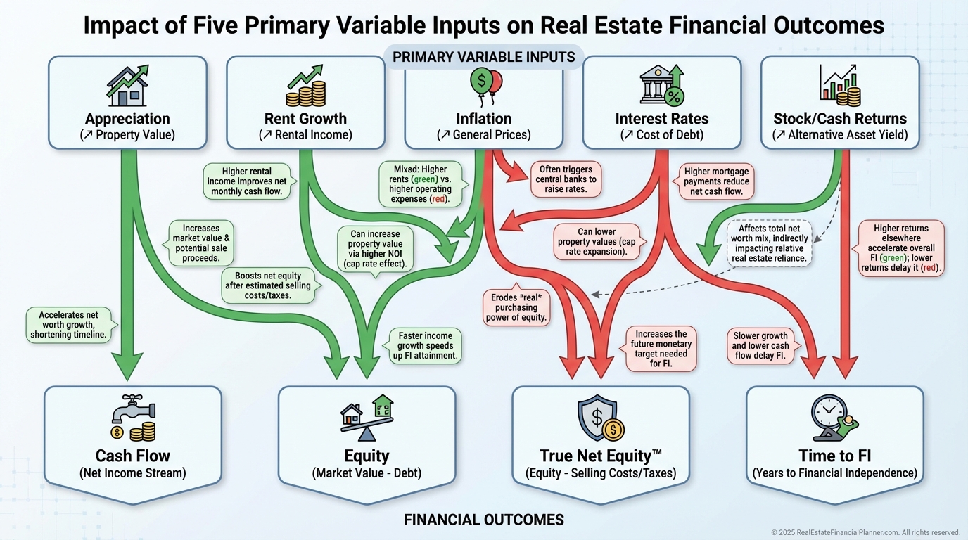
The Inputs That Actually Move Your Outcomes
When I model plans, these inputs do the heavy lifting:
•
Property appreciation rate
•
Rent appreciation rate
•
Inflation
•
Mortgage interest rates (until you fix a loan)
•
Stock/bond/cash returns
If we want to get “freaky accurate,” we can also vary taxes, insurance, maintenance, CapEx, and vacancy.
But start with the big five.
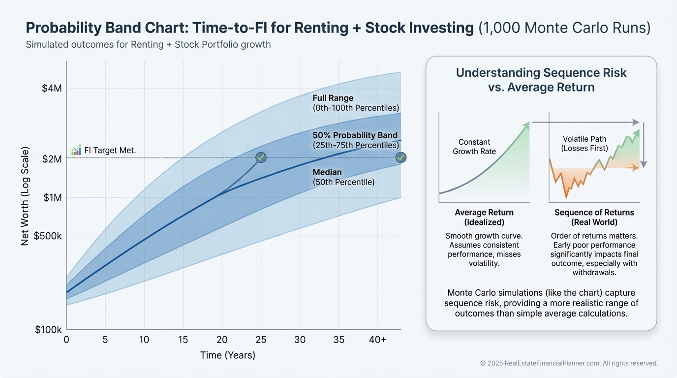
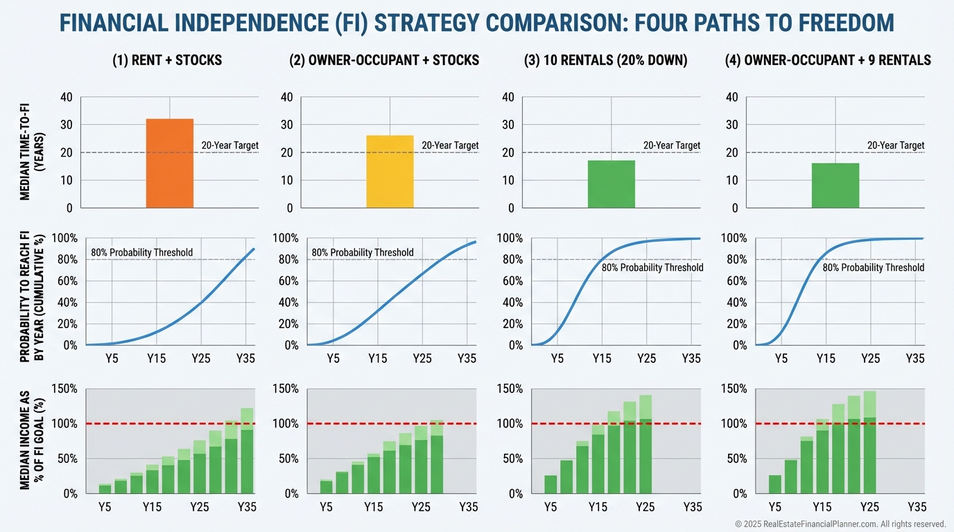
A Simple Baseline: Renting and Investing Only in Stocks
Start simple.
Assume you rent your home and invest 10% of income into a diversified stock portfolio averaging 8% over the long run.
With static assumptions, you might “hit FI” in roughly 53 years.
But markets don’t hand you 8% each year.
When I rerun this scenario through 1,000 Monte Carlo paths, the FI date spreads out.
In strong sequences, you cross FI a decade earlier.
In poor sequences, you may still be short at year 60.
The lesson: average returns aren’t your experience; sequences are.
Buying the Home You Live In
Now let’s buy an owner-occupant property with 5% down.
Under static assumptions, you reach FI about 15.5 years faster than renting + stocks.
Monte Carlo still shows a wide range, but two forces help:
•
You eventually eliminate your largest expense when the mortgage is paid.
•
The FI target drops because your housing cost falls in retirement.
When I coach clients, I show how locking a 30-year fixed rate caps one of the most volatile line items you have.
Buying 10 Rentals with 20% Down
Let’s level up.
You continue renting personally, but you buy up to ten rentals with 20% down whenever you have the cash, investing the rest in stocks.
With static inputs, clients often reach FI ~31 years in.
That’s about 18.5 years faster than renting + stocks and about 3 years faster than buying only an owner-occupant home.
The gap grows over time as rents rise and loans amortize.
Monte Carlo adds realism: sometimes you buy in soft markets with high rates and thin cash flow; sometimes you catch great appreciation and lower rates.
The spread of outcomes is larger, but so is the upside.
Owner-Occupant + Nine 20% Down Rentals
This hybrid usually improves both speed and probability.
You stabilize your personal housing cost, then scale rentals.
In my models, the median time-to-FI is faster than either strategy alone, and the probability curve shifts left and up.
Left means earlier.
Up means more runs succeed by each date.
The Nomad™ Strategy
Nomad™ is simple and powerful.
You buy with 5% down as an owner-occupant, live there at least a year (as your lender requires), then move into the next 5% down property and convert the last one to a rental.
Repeat until you hold a portfolio you like.
You acquire rentals with lower down payments, typically better rates, and often better DSCR because you lived in the property first and improved it while there.
Under static assumptions, Nomad™ was about 58 months faster to FI in my sample plan.
Monte Carlo typically shows it’s both faster and more probable than the other approaches tested.
What I Model, Check, and Avoid in Client Plans
When I build plans with clients, I model:
•
Appreciation and rent growth as distributions, not points
•
Mortgage rates as variable until locked, then fixed
•
Inflation that drifts and spikes, not a flat CPI
•
Stock/bond/cash returns with realistic volatility and correlation
I check:
•
Liquidity and reserves through stress windows
•
Debt-to-income bottlenecks during the acquisition phase
•
Cash flow under higher rate / lower rent growth paths
•
Tax-sensitive outcomes using True Net Equity™
I avoid:
•
Overweighting cash-on-cash in year one
•
Ignoring refinancing and rate-buydown options
•
Counting on perfect BRRRR appraisals or zero-vacancy
•
Assuming constant capex; roofs don’t read your spreadsheet
Beyond “How Fast to FI”: Two Standards That Matter
Speed is only half the story.
Your standard of living after FI matters.
If you need $10,000/month to be FI but your portfolio produces $20,000, you can live better, reinvest, or derisk.
Probability matters too.
A strategy that averages one year faster but doubles your failure risk is often a poor trade.
Monte Carlo exposes both.
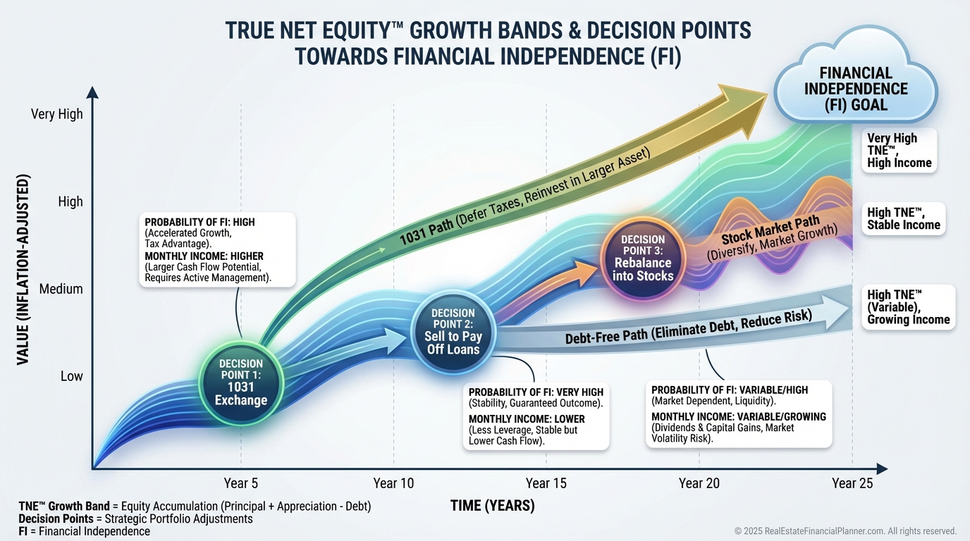
Using True Net Equity™ and Probability Bands
True Net Equity™ adjusts your “paper equity” for selling costs, transaction friction, and taxes.
It’s what you could actually redeploy.
In simulations, I track True Net Equity™ distributions over time to see when 1031s, free-and-clear payoffs, or strategic sales make sense.
Then I test how those moves shift FI probability by year.
That’s how we decide whether to sell three rentals in year 18 to pay off two, or just keep all ten.
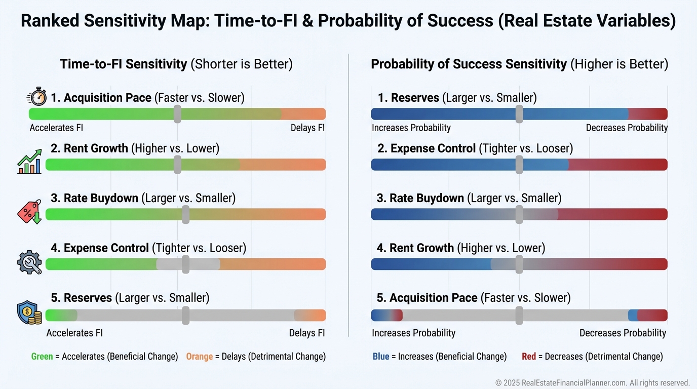
Sensitivity: What Moves the Needle Most?
Clients always ask, “What should I optimize first?”
In most plans, the big levers are:
•
Interest rate at purchase (buydowns can be huge)
•
Acquisition pace and price discipline
•
Rent growth versus expense creep
•
Reserves that survive rate shocks and vacancy
I run one-variable sensitivity sweeps to show which lever gives the largest improvement in time-to-FI and probability.
Then we prioritize action steps you control.
Practical Modeling Tips from the Trenches
A few rules I live by when I model:
•
Model rate volatility until the day you lock.
•
Use rent growth below appreciation in conservative plans.
•
Cap rent-to-price compression; it doesn’t expand forever.
•
Keep 6–12 months of personal and property reserves, tested across bad sequences.
•
Don’t count tax benefits you can’t actually use.
•
Reforecast annually; your plan should age with you.
When I rebuilt after a business failure in my 20s, the lesson was simple: survive first.
Monte Carlo helps you see survival odds before you wager your future.
Action Steps with RealEstateFinancialPlanner.com
•
Define your FI target in today’s dollars. Then inflation-adjust it in the plan.
•
Choose your base strategy: owner-occupant, 20% down rentals, owner-occupant + rentals, or Nomad™.
•
Turn on Monte Carlo for appreciation, rents, inflation, rates, and market returns.
•
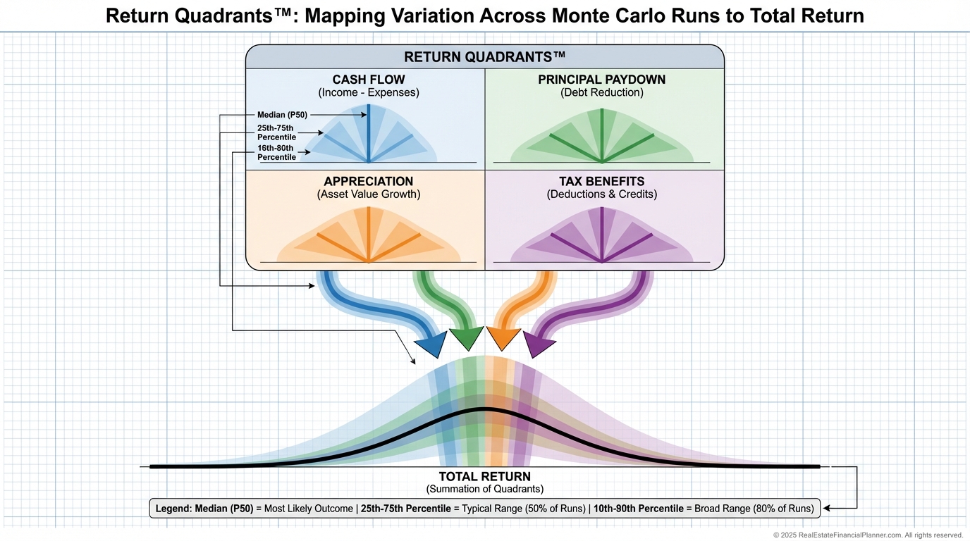
Track Return Quadrants™ and True Net Equity™ over time.
•
Review FI probability by year. If the curve is too flat or too low, adjust levers.
•
Re-run annually and after major market shifts.